Time Domain |
| It is a process that its value varies with time. For instance, consider the temperature in New York City. If we continually measure and store the temperature in a magnetic tape, then it could be said that the temperature in New York City is the time domain. That is, give a specific time value; it is possible to know the temperature. Humans are used to understand and observe this kind of processes. |
Frequency Domain |
| It is a process that exhibits some sort of periodic behavior. To measure this periodic behavior, it is important to know how many periodic events occur per unit of time. The frequency of an event indicates the number of repetitions of a periodic event and it described in Hertz (cycles per seconds). Periodic processes are better understood in the frequency domain. |
Fourier Transform |
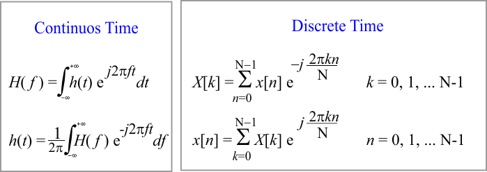
| A (physical) process can be seen and analyzed in the time domain or in the frequency domain. The Fourier Transform is used to transform a process from the time domain to the frequency domain. Once the transformation has been applied, time information is hidden and cannot be easily observed. It cannot be said that time information is lost because it is possible to recover the original time domain observation using the Inverse Fourier Transform. The equations below show the Fourier Transform equations where f is the frequency in Hz, and t is the time in seconds. |
| Tip |
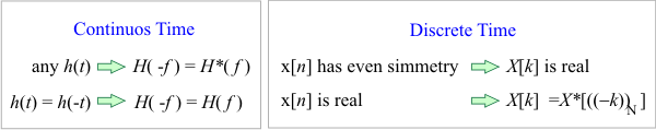
| In some applications h(t) is purely real and the following symmetry properties applied: |
| Problem 1 |
| Prepare a one page summary of the Discrete Fourier Transform including the transform pairs and theorems listed: time scaling, frequency scaling, time shifting, frequency shifting, duality, convolution, correlation theorem, Wiener-Khinchin theorem, and Parsevals theorem. An excellent reference is: Discrete-Time Signal Processing, A. V. Oppenheim and Ronald W. Schafer. |
Windowing |
| Windowing is a method that is applied to a signal before taking its Fourier Transform. Windowing MUST be used when the value of the signal at the beginning is different from the value of the signal at the end. Windowing is used to reduce the appearance of new frequencies due to spectral leakage. For a sine wave of frequency w the leakage tends to be worst near w and least at frequencies farthest from w. In a classification problem, applying a window to the signal before using the Fourier Transform may increase the accuracy of the classification. |
Window Types |
| There are several windows that can be used to reduce leakage. A window length M must equal to length of the input series (x[n]). Some of them are shown below. |
| Problem 2 |
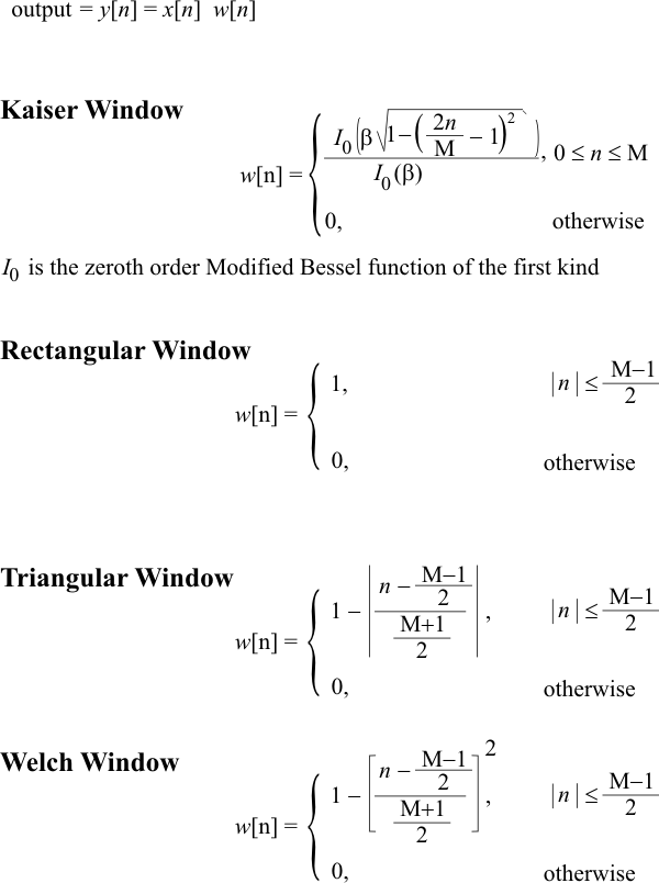
| Create a Neural Lab project called Fourier with Main file only. Plot the Welch Window for a series of length 512 using Neural Lab. |
| Fourier\WelchWindow.lab |
| //___________________________________________________ 1. Compute Window int M = 512; Vector n; n.CreateSeries(0, M-1, M); Vector tmp = (n - (M-1)/2)/((M+1)/2); Vector w = 1 - tmp*tmp; //___________________________________________________ 2. Graph XyChart chart; chart.SetCaption("n", false, "Welch", false); chart.AddGraph(n, w, "Welch Window", 2, 1, 0, 255, 0); chart.SetLimits(0.0, M, 0.0, 1.0); chart.SetColorMode(2); chart.SaveAndShow(); |
| Problem 3 |
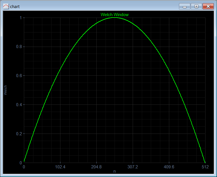
| if x[n] = sin[n/8], compute and plot y[n] = w[n] x[n] using the Welch Window. Suppose that the length of x is 512. |
| Fourier\WelchSine.lab |
| //___________________________________________________ 1. Compute Window int M = 512; Vector n; n.CreateSeries(0, M-1, M); Vector tmp = (n - (M-1)/2)/((M+1)/2); Vector w = 1 - tmp*tmp; Vector x = sin(n/8); Vector y = w*x; //___________________________________________________ 2. Graph XyChart chart; chart.SetCaption("n", false, "Welch", false); chart.AddGraph(n, y, "y", 2, 1, 0, 255, 0); chart.SetLimits(0.0, M, -1.0, 1.0); chart.SetColorMode(2); chart.SaveAndShow(); chart.SavePDF(0.0); |
| Problem 4 |
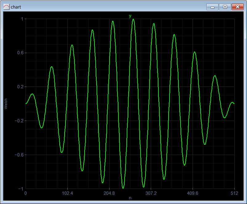
| Plot the spectrum of the signal in the previous problem using Neural Lab. Use the spectrum function. |
| Fourier\Spectrum.lab |
| //___________________________________________________ 1. Compute Window int M = 512; Vector n; n.CreateSeries(0, M-1, M); Vector tmp = (n - (M-1)/2)/((M+1)/2); Vector w = 1 - tmp*tmp; Vector x = sin(n/8); Vector y = w*x; Vector Y = spectrum(y); //___________________________________________________ 2. Graph XyChart chart; chart.SetCaption("n", false, "Welch", false); chart.AddGraph(n, Y, "Y", 2, 1, 0, 255, 0); chart.SetLimits(0.0, M/2, 0.0, Y.GetMax()); chart.SetColorMode(2); chart.SaveAndShow(); chart.SavePDF(0.0); |
| Problem 5 |
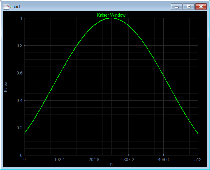
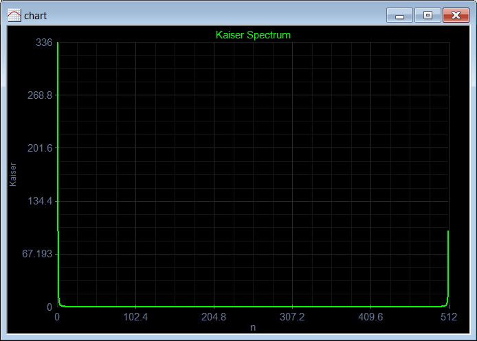
| Using Neural Lab: (a) Plot the Kaiser Window for a series of length 512 using the function Vector.CreateKaiser. Use β = 3.3; (b) Plot the FFT of the Kaiser Window. |
| Fourier\KaiserA.lab |
| //___________________________________________________ 1. Compute Kaiser window Vector w; w.CreateKaiser(3.3, 512); //___________________________________________________ 2. Graph XyChart chart; chart.SetCaption("n", false, "Kaiser", false); chart.AddGraphY(w, "Kaiser Window", 2, 1, 0, 255, 0); chart.SetLimits(0.0, 512, 0.0, 1.0); chart.SetColorMode(2); chart.SaveAndShow(); chart.SavePDF(0.0); |
| Fourier\KaiserB.lab |
| //___________________________________________________ 1. Compute Kaiser window Vector w; w.CreateKaiser(3.3, 512); Vector W = abs(fft(w)); //___________________________________________________ 2. Graph XyChart chart; chart.SetCaption("n", false, "Kaiser", false); chart.AddGraphY(W, "Kaiser Spectrum", 2, 1, 0, 255, 0); chart.SetLimits(0.0, 512, 0.0, W.GetMax()); chart.SetColorMode(2); chart.SaveAndShow(); chart.SavePDF(0.0); |
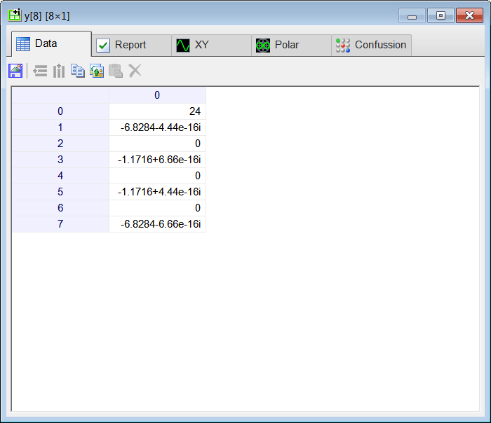
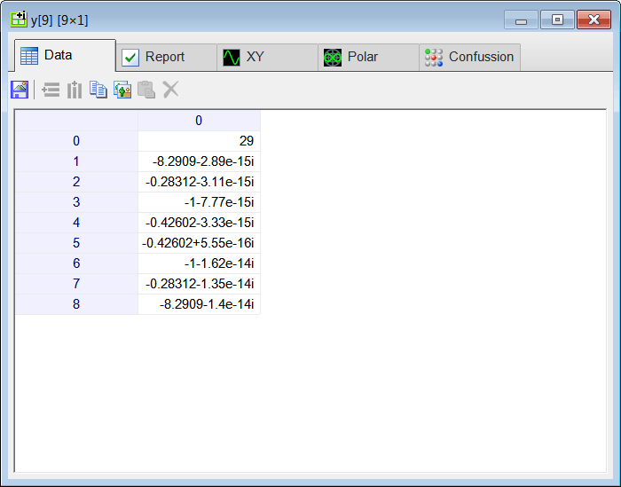
| Problem 6 |
Using Neural Lab find the FFT of:
|
| Fourier\FftTest1a.lab |
| Vector x; x.Create(8); x[0] = 1; x[1] = 2; x[2] = 3; x[3] = 4; x[4] = 5; x[5] = 4; x[6] = 3; x[7] = 2; ComplexVector y = fft(x); x.Save(); y.Save(); |
| Fourier\FftTest1b.lab |
| Vector x; x.Create(9); x[0] = 1; x[1] = 2; x[2] = 3; x[3] = 4; x[4] = 5; x[5] = 5; x[6] = 4; x[7] = 3; x[8] = 2; ComplexVector y = fft(x); x.Save(); y.Save(); |
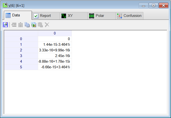
| Problem 7 |
Using Neural Lab find the FFT of:
|
| Fourier\FftTest2a.lab |
| Vector x; x.Create(12); x[0] = 0; x[1] = 1; x[2] = 2; x[3] = 3; x[4] = 2; x[5] = 1; x[6] = 0; x[7] = -1; x[8] = -2; x[9] = -3; x[10] = -2; x[11] = -1; ComplexVector y = fft(x); x.Save(); y.Save(); |
| Fourier\FftTest2b.lab |
| Vector x; x.Create(6); x[0] = 0; x[1] = 1; x[2] = 1; x[3] = 0; x[4] = -1; x[5] = -1; ComplexVector y = fft(x); x.Save(); y.Save(); |
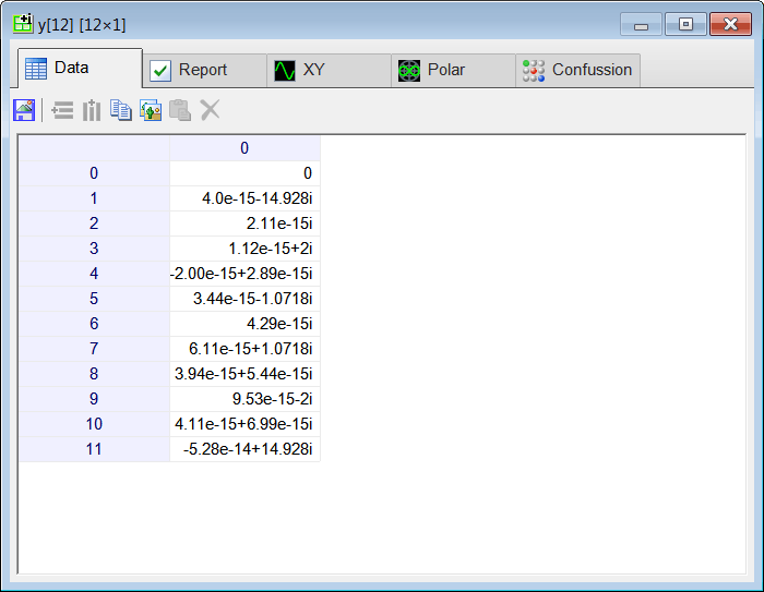
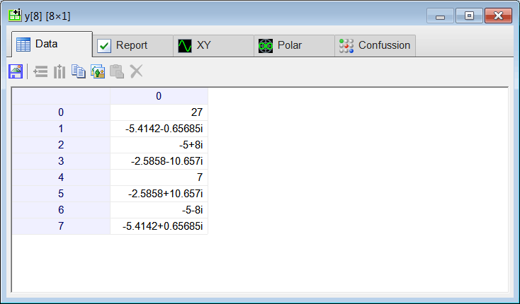
| Problem 8 |
| Using the series x[n] = 1, 2, 3, 7, 5, -1, 8, 2; show the conjugate property. In this case, as x is real, its conjugate is the same as x. Thus, if the complex conjugate of the FFT of x is reversed, we get the FFT of x. In other words, for real signals, the FFT is symmetric complex conjugated. |
| Fourier\ConjugateTest.lab |
| Vector x; x.Create(8); x[0] = 1; x[1] = 2; x[2] = 3; x[3] = 7; x[4] = 5; x[5] = -1; x[6] = 8; x[7] = 2; ComplexVector y = fft(x); x.Save(); y.Save(); |
| Problem 9 |
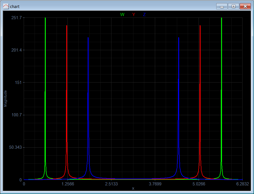
| Plot the magnitude of the FFT of w=sin(50x), y=sin(100x) and z=sin(150x). |
| Fourier\SinTest.lab |
| //___________________________________________________ 1. w, y and z Vector x; x.CreateSeries(0, 6.2832, 512); ComplexVector w = fft(sin(50*x)); ComplexVector y = fft(sin(100*x)); ComplexVector z = fft(sin(150*x)); // Vector magW = abs(w); Vector magY = abs(y); Vector magZ = abs(z); //___________________________________________________ 2. Graph XyChart chart; chart.SetCaption("x", false, "Magnitude", false); chart.AddGraph(x, magW, "W", 2, 1, 0, 255, 0); chart.AddGraph(x, magY, "Y", 2, 1, 255, 0, 0); chart.AddGraph(x, magZ, "Z", 2, 1, 0, 0, 255); chart.SetLimits(0.0, 6.2832, 0.0, magW.GetMax()); chart.SetColorMode(2); chart.SaveAndShow(); chart.SavePDF(0.0); |
| Problem 10 |
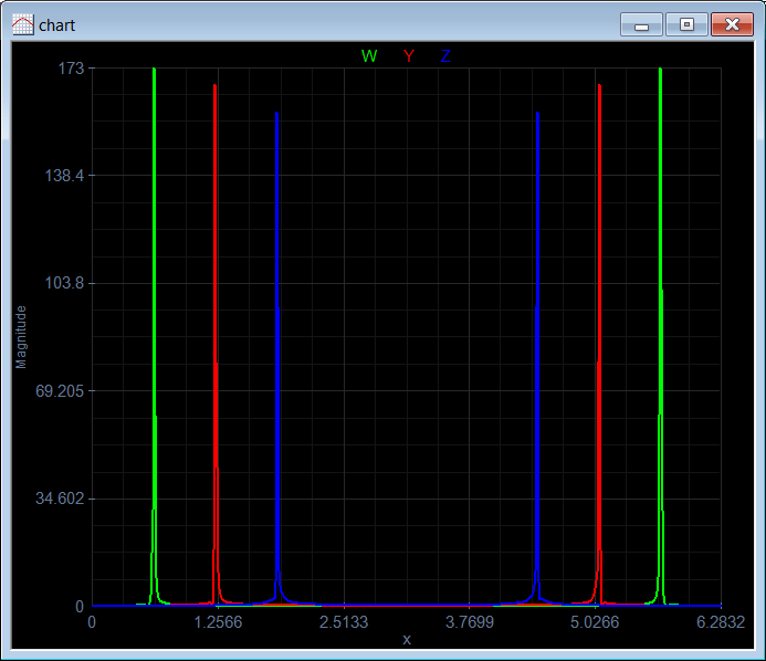
| Repeat the same problem using a Kaiser window with beta=3. |
| Fourier\KaiserTest.lab |
| //___________________________________________________ 1. w, y and z Vector x; x.CreateSeries(0, 6.2832, 512); Vector window; window.CreateKaiser(3.0, 512); ComplexVector w = fft(window*sin(50*x)); ComplexVector y = fft(window*sin(100*x)); ComplexVector z = fft(window*sin(150*x)); // Vector magW = abs(w); Vector magY = abs(y); Vector magZ = abs(z); //___________________________________________________ 2. Graph XyChart chart; chart.SetCaption("x", false, "Magnitude", false); chart.AddGraph(x, magW, "W", 2, 1, 0, 255, 0); chart.AddGraph(x, magY, "Y", 2, 1, 255, 0, 0); chart.AddGraph(x, magZ, "Z", 2, 1, 0, 0, 255); chart.SetLimits(0.0, 6.2832, 0.0, magW.GetMax()); chart.SetColorMode(2); chart.SaveAndShow(); chart.SavePDF(0.0); |
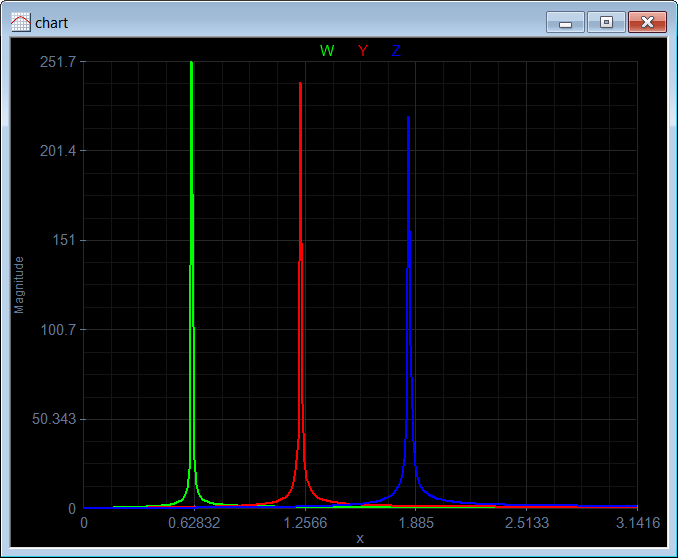
| Problem 11 |
| For real signals, the FFT is symmetric. The spectrum function returns the magnitude of only half of the frequencies. Repeat problem 9 using spectrum instead of fft. |
| Fourier\SinSpectrum.lab |
| //___________________________________________________ 1. w, y and z Vector x; x.CreateSeries(0, 6.2832, 512); Vector W = spectrum(sin(50*x)); Vector Y = spectrum(sin(100*x)); Vector Z = spectrum(sin(150*x)); //___________________________________________________ 2. Graph XyChart chart; chart.SetCaption("x", false, "Magnitude", false); chart.AddGraph(x, W, "W", 2, 1, 0, 255, 0); chart.AddGraph(x, Y, "Y", 2, 1, 255, 0, 0); chart.AddGraph(x, Z, "Z", 2, 1, 0, 0, 255); chart.SetLimits(0.0, 3.1416, 0.0, W.GetMax()); chart.SetColorMode(2); chart.SaveAndShow(); chart.SavePDF(0.0); |
Wintempla and Digital Signal Processing |
| Most of the functions to perform Digital Signal Processing in Wintempla are inside the the Math::Dsp class. |
| Problem 12 |
| Create a Dialog application called FftApp using Wintempla to compute the Fast Fourier Transform of a series. |
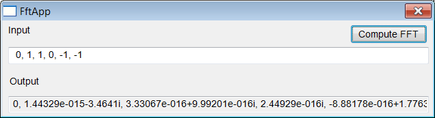
| FftApp.cpp |
| #include "FftApp.h" int APIENTRY wWinMain(HINSTANCE hInstance, HINSTANCE , LPTSTR cmdLine, int cmdShow){ FftApp app; return app.BeginDialog(IDI_FFTAPP, hInstance); } void FftApp::Window_Open(Win::Event& e) { } void FftApp::btComputeFft_Click(Win::Event& e) { //_________________________________ Extract the data from the GUI valarray<complex<double> > x; valarray<complex<double> > X; Sys::Convert::ToVector(tbxInput.Text, x); const int len = x.size(); //__________________________________ Perform the transformation if (Math::Dsp::IsPowerOfTwo(len) == true) { Math::Dsp::Fft(x, X, false); } else { Math::Dsp::FourierTransform(x, X, false); } //___________________________________ Display the result wstring text; Sys::Convert::ToString(X, text); tbxOutput.Text = text; } |
Fast Fourier Transform with Microsoft Excel |
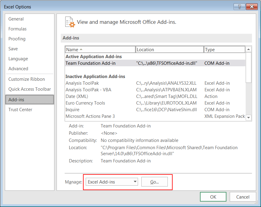
| In order to compute a FFT using Microsoft Excel, you must activate Data Analysis in the Data tab. Use File > Options > Add-ins to activate Data Analysis as shown below. Click on the Go button. A fin de calcular una FFT usando Microsoft Excel, usted debe activar Análisis de Datos en la pestaña de Datos. Use Archivo > Opcions de Excel > Complementos para activar Análisis de Datos como se muestra debajo. Haga clic en el botón de Ir. |
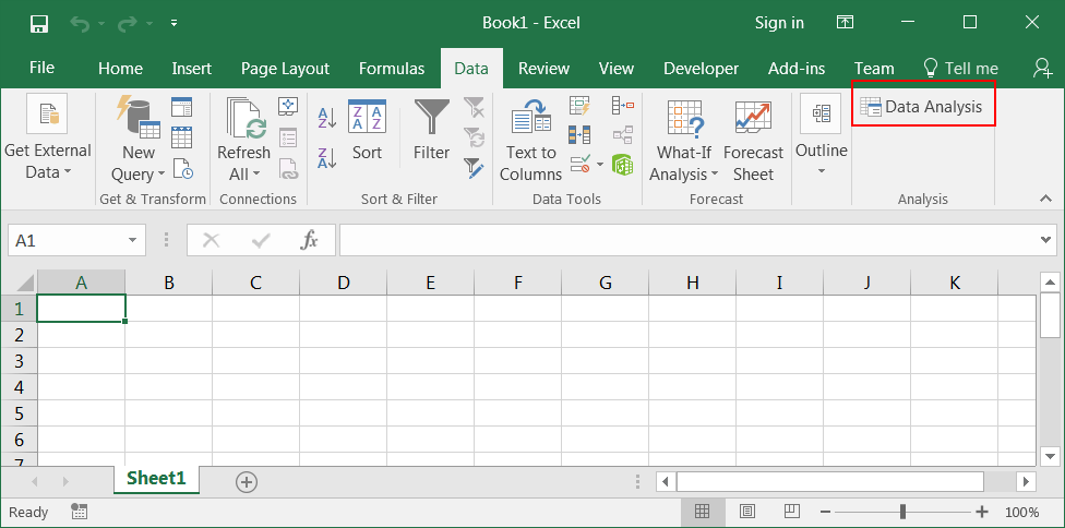
| Step A |
| Open Microsoft Excel. Then click on File > Options > Add-ins to activate Data Analysis as shown below. Click on the Go button. Abra Microsoft Excel. Entonces haga clic en Archivo > Opciones de Excel > Complementos para activar Análisis de Datos como se muestra debajo. Haga clic en el botón de Ir. |
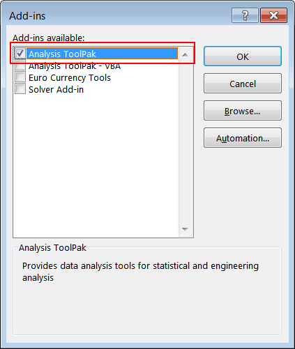
| Step B |
| Check Analysis ToolPak and click the OK button. Marque Herramientas para Análisis y haga clic en el botón de Aceptar. |
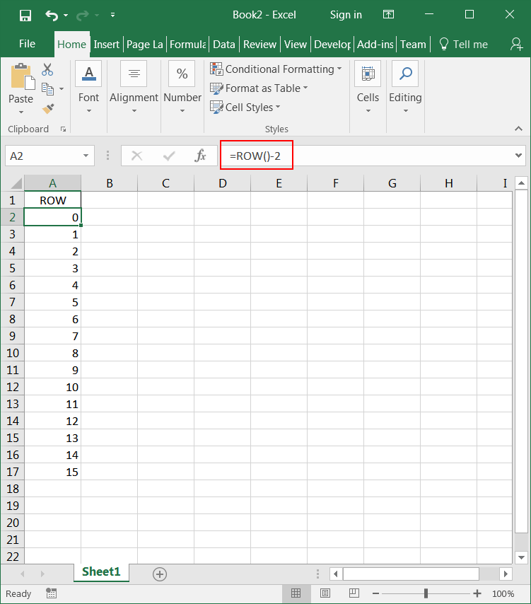
| Problem 13 |
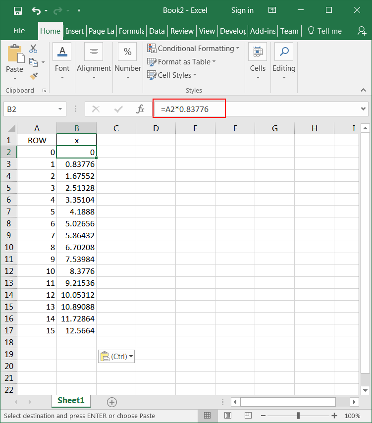
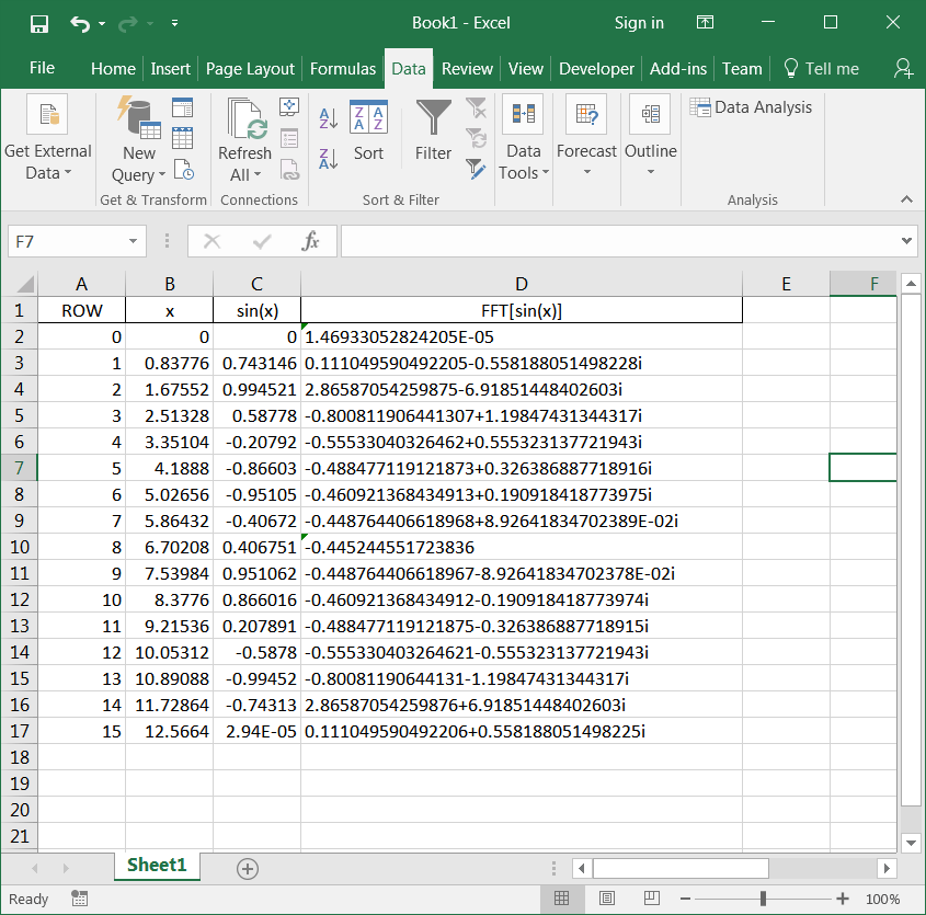
| Open Microsoft Excel. Using your Microsoft Excel skills create the first column using the formula as shown. Abra Microsoft Excel. Usando sus habilidades en Microsoft Excel cree la primera columna usando la fórmula como se muestra. |
| Step A |
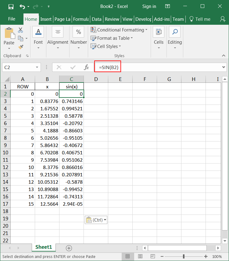
| Create the second column using the formula as shown. Cree la segunda columna usando la fórmula como se muestra. |
| Step B |
| Create the third column using the formula as shown. Cree la tercera columna usando la fórmula como se muestra. |
| Step C |
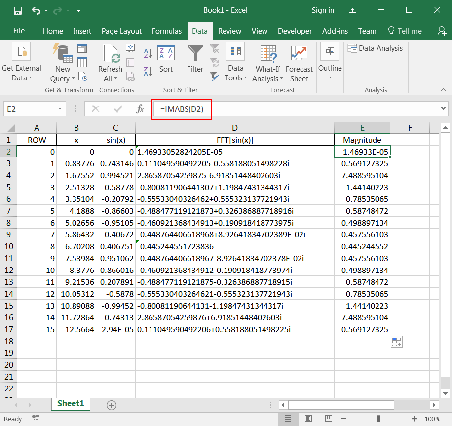
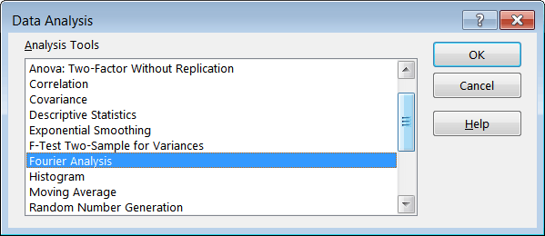
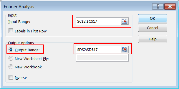
| To complete the fourth column, click on Data Analysis on the Data tab. Then select Fourier Analysis, and click the OK button. Set the input and output options as shown, and click OK. Para completar la cuarta columna, haga clic en Análisis de Datos en la pestaña de Datos. Entonces seleccione Análisis de Fourier, y haga clic en el botón de Aceptar. Fije las opciones de entrada y salida como se muestra, y haga clic en Aceptar. |
| Step D |
| Create the fifth column using the formula as shown. Cree la quinta columna usando la fórmula como se muestra. |